
Enabling Bad Behavior: The Federal Reserve’s Municipal Liquidity Facility in Retrospect
Executive Summary
In response to the COVID-19 pandemic, the Coronavirus Aid, Relief, and Economic Security (CARES) Act greatly expanded government intervention in the economy. Among many hasty creations of March 2020 were the Federal Reserve Emergency Lending Facilities. One of these lending facilities, the Municipal Liquidity Facility (MLF), provided aid to fiscally distressed state and local governments. For the first time in its history, the Federal Reserve purchased municipal bonds.
By the time the MLF closed, only the State of Illinois and the New York Metropolitan Transportation Authority (MTA), both of which were fiscally weak before 2020, had accessed MLF loans. While both entities paid back the loan before the deadline, the MLF loan did not require either Illinois or the MTA to make any changes to spending or debt accumulation. The case studies of Illinois and the MTA show the loans barely improved cash flow, but did encourage rent-seeking among fiscally distressed states and the creation of a monetary commons.
To avoid recreating the state budget strains that created the demand for something like the MLF, several policy solutions are offered. First, states must reduce dependence on federal transfers. Second, policymakers in both fiscal and monetary spaces must commit to a monetary rule and end credit allocation. Third, state policymakers must commit to stringent fiscal rules to decrease spending and limit how much a state can borrow. Fourth, “off-budget enterprises” that enjoy taxpayer support without being subjected to the same budget rules as official government entities (such as mass transit authorities) must either be brought “on-budget” and subjected to state fiscal rules or relinquish state support.
Key Points
- The Municipal Liquidity Facility (MLF) was the result of three related factors:
- states’ eagerness to access federal funds
- federal policymakers’ eagerness for influence over state affairs
- policy changes in the Federal Reserve operating framework that enable it to engage in fiscal policy, rather than the monetary policy which is its domain.
- State reliance on transfer payments from the federal government dramatically increased beginning in the 1960s. By the mid-1990s, federal expenditures were the second-largest input to state budgets.
- The Federal Reserve (the Fed) has always been susceptible to mission creep, but the opportunity cost of mission creep was significantly lowered by Fed policy changes in 2008, specifically changing to the “floor system” which allows the central bank to buy assets with newly created money, in order to afford Congress’s spending policies.
- Bad behavior on the part of federal, state, and monetary officials was actively encouraged.
- Both the State of Illinois and the New York Metropolitan Transportation Authority were struggling financially prior to 2020 and have not made any substantial reforms to improve fiscal health after receiving loans from the MLF.
- The creation and implementation of the MLF creates a moral hazard for state budgeting officials, who may bank on the probability of future bailouts.
- Structural reforms are necessary at the state and federal level to discourage Fed mission creep, avoid further Fed interventions in the municipal bond market, and reduce the chances of future state bailouts.
Introduction
In 2021, the Sound Money Project at The American Institute for Economic Research published a paper titled, “The Federal Reserve’s Response to the COVID-19 Contraction: An Initial Appraisal.”[1] In that appraisal, Cachanosky et al. concluded:
“Although some facilities likely helped to promote general liquidity, others were primarily intended to allocate credit, which blurs the line between monetary and fiscal policy. These credit allocation facilities were unwarranted and unwise.”[2]
Among the lending facilities Cachanosky et al examined was the Municipal Liquidity Facility (MLF), which was aimed at providing credit to state and local government borrowers. Only two entities accessed the MLF during its existence: the State of Illinois and the New York Metropolitan Transportation Authority (MTA).
This paper will argue that the creation of the MLF, specifically, was “unwarranted and unwise.” First, I will provide a brief overview of federal transfers to the states, which paved the way for the CARES Act in 2020 and created incentives for state policymakers to seek transfer payments from the federal government. Second, I will review the literature which shows how the changes in the Federal Reserve’s Operating Framework in 2008 (specifically the change to a floor system) created a low opportunity cost for mission creep. Third, I will outline how the factors from the first two sections created incentives for monetary intervention in the municipal bond market on the part of state and federal policymakers as well as Federal Reserve officials. Fourth, I will outline the design and operations of the Municipal Liquidity Facility. Fifth, I will draw on The Hoover Institution State Fiscal Strength Indicators to show how Illinois and the MTA had low fiscal strength prior to 2020 and in the years to follow, indicating that the MLF loans provided little to no improvements for these entities. Sixth, I will discuss how these factors create moral hazards among state governments and incentivize future Fed interventions in the municipal bond market. Seventh, I will briefly offer options for fiscal and monetary policy reform to prevent future interventions from another MLF.
Public Debt Strained State Budgets Long Before 2020
Between the 1960s and the 1990s, while states were becoming increasingly dependent upon federal funds, they were also taking on debt. This came in two forms: bonded obligations and unfunded liabilities.
Bonded obligations are what’s commonly known as “public debt.” States and municipalities issue bonds for various purposes, bond investors purchase the bonds, and the government pays the bond investors back with interest using taxpayer dollars. These debt payments can be tracked in state and local financial reports and by the Municipal Securities Rating Board (MSRB).
As described by James Buchanan, when a government takes on debt, it shifts the tax burden from the present to future generations. Taxpayers in the present enjoy the increased spending without a tax hike. Although bond investors buy bonds, they only do so because they can expect to be paid back with interest. Future generations are the ones paying for the past spending with a “genuine sacrifice” to their income. [3]
A liability for a public pension or other post-employment benefit (OPEB) plan is a promised benefit to public employees (such as a pension or retiree health insurance) that is expected to be paid out when that public employee retires. When benefit plan assets (combined contributions from employees, taxpayer dollars, and investment returns) are less than total promised benefits, the remaining promised benefits are considered “unfunded liabilities.” Totalling up these unfunded liabilities is far more difficult than determining total bonded obligations.
As my colleague Ryan Yonk and I discuss in Understanding Public Debt, to determine whether or not a benefit plan has unfunded liabilities, one must calculate the present value of the total liabilities.[4] The present value shows the value today of those promised benefits in the future, which depends on what economists refer to as a discount rate.[5] The higher the discount rate, the lower the present value and vice versa. The present value of those promised benefits is also sensitive to discount rate changes. Even if the discount rate changes by fractions of a percentage point, the present value of unfunded liabilities could change by millions of dollars. While some researchers (including myself) suggest using lower discount rates to determine the present value of unfunded liabilities, this paper will rely on unfunded liability estimations based on government accounting standards.[6]
Data show the status of outstanding state debt for FY 2019 (the last full fiscal year prior to the COVID-19 economic downturn) was well into the trillions of dollars. Outstanding state bonded obligations totaled $1.16 trillion (2019 dollars).[7] Unfunded pension liabilities estimated to be $1.3 trillion and unfunded OPEB liabilities were estimated to be $660.7 billion (both in 2019 dollars).[8],[9]
States Are Reliant on Federal Tax Dollars to Cover Spending
Throughout American history, the federal government has exerted some influence in state and local government policy by giving and withholding federal transfers.[10] The most relevant portion of that history to this paper begins in the 1960s, with the creation of the Great Society programs under President Johnson. From 1960-1970, federal grants to state and local governments tripled from 132 in 1960 to 387 in 1968.[11] In the 1970s, the federal government shifted from narrowly focused categorical grants, with strict guidelines on how funds must be used, to block grants and revenue sharing that allowed state and local governments greater discretion over how federal money was spent. [12] During the 1980s, grants were further consolidated, but federal transfers to state and local governments increased.State governments were empowered to raise spending on the backs of federal taxpayers in other states, and the federal government was empowered with greater control over state and local affairs. [13]
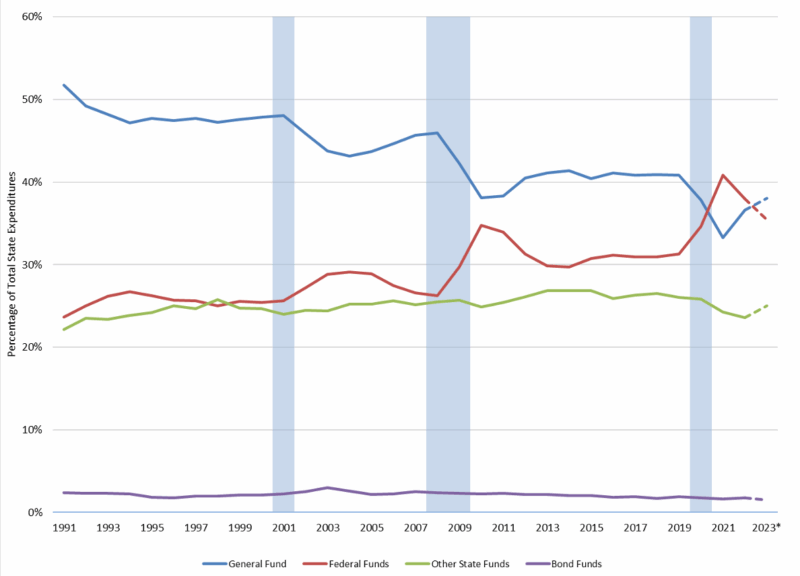
By 1991, federal funding comprised almost a quarter of all state expenditures.[14] As Figure 1 shows, the Great Recession cemented federal transfers as the second-largest source of funding for state governments. State policymakers steadily increased spending while passing the cost onto federal taxpayers in other states. Federal policymakers increased their own influence over affairs which would otherwise be left entirely to state and local governments or the private sector, by carefully crafting the terms and conditions for receiving these federal transfers. [15]
Figure 1: State Expenditures (Capital Inclusive) by Source as a Percentage of Total State Expenditures (50 State Average)

Sources: Earle and Savidge, “Fiscal Federalism Turned Upside Down,” National Association of State Budget Officers (NASBO) State Expenditure Report 2023, and NASBO State Expenditure Report Historical Data.
Notes: 2023 totals are projected. Shaded areas indicate periods of recession.
Ultimately, the dramatic increase in federal transfers to the states during the Great Recession reassured state policymakers that they could look to federal policymakers to cover budget shortfalls, which played out during 2020. State policymakers padded state budgets with federal taxpayer dollars to avoid making tough budgeting decisions such as tax increases or spending cuts, both of which risk voter backlash. This arrangement between the federal and state governments in 2008 also set the stage for state policymakers to alleviate budget stress with something like the Municipal Liquidity Facility.
Changes in the Federal Reserve’s Operating Framework Encourage Mission Creep
The Great Recession also brought about great changes in monetary policy. Following the financial crisis, the Federal Reserve radically altered its operating framework from what was known as a corridor system to a floor system. Under the pre-2008 corridor system, the Federal Reserve influences the federal funds rate (the interest rate at which depository institutions trade balances held at the Federal Reserve Banks with each other overnight) through open-market operations. These involve the Federal Reserve injecting or withdrawing reserves to shift supply of these balances, keeping the market rate between the discount rate and the interest rate on reserves (IOR). The system requires reserve scarcity for the Fed to steer interest rates effectively.[16] When the Fed adopted the floor system in 2008, the banking system was flooded with reserves. Instead of engaging in open market operations (which have lost their potency in this system), the Fed influences the federal funds rate by adjusting the interest rate on reserves, which has now become the binding anchor.[17]
Consequently, the post-2008 floor system allowed the Fed to expand its balance sheet via quantitative easing (QE) without triggering inflation. Selgin (2020) notes that this “decoupling” of reserve quantity enabled what he calls “fiscal QE,” or when the central bank buys assets with newly created money, in order to afford Congress’s spending policies.[18] Selgin, echoing Plosser (2012), further cautions that this blurring of fiscal and monetary functions compromises Fed independence and invites future political meddling.[19],[20] In a 2020 episode of the podcast Macro Musings, Selgin also warned against the potential dangers of flexible average inflation targeting (FAIT), which was adopted after the onset of the COVID-19 pandemic. He commented, “[The Fed] has given itself a larger number of degrees of freedom to do whatever the heck it wants to do. Now, conceivably, it could improve things. But it’s hardly obvious that it will.”[21]
Since 2008, Rouanet and Salter (2024) note that the Fed has expanded its objectives beyond the “dual mandate” and weighed in on various social issues by engaging in credit allocation, pushed both by external political pressure and internal demand from those at the Fed itself. This expansion, they argue, comes from “the floor system and unconventional monetary policies since 2008” which lowered the opportunity cost of mission creep.
Furthermore, findings from Custinger (2025) confirm Selgin’s 2020 warning about FAIT. Though intended to compensate for past inflation undershoots by tolerating above-target inflation, FAIT lacked a similar mechanism to counteract overshoots, effectively guaranteeing prolonged inflation.[22] He also notes that this asymmetry encouraged the Fed’s delayed policy response to post-2020 inflation, undermining long-term price stability, and further exposing the Fed’s framework to mission creep.
The development of Fed policy since 2008 and in the lead-up to 2020 signals a strong drift toward central bank activism.
The MLF: The Culmination of Federal Transfers and Fed Mission Creep
With the passage of the CARES Act came the largest expansion of the Federal Reserve’s authority since the Great Recession. While the Federal Reserve has the authority to purchase state and municipal bonds under Section 14(2)(b) of the Federal Reserve Act, Rouanet and Salter (2024) note, “it had historically been reluctant to do so.”[23] Changes to the Federal Reserve operating frameworks discussed in the previous section and volatility in the municipal bond market eroded that reluctance. With the encouragement of Treasury officials, the MLF was created under Section 13(3) of the Federal Reserve Act, granting the Federal Reserve emergency lending authority in necessary circumstances to a “special purpose vehicle.”[24]
The MLF Term Sheet provided guidelines for what bonded obligations the MLF can buy, which state and local entities can sell bonded obligations to the MLF, and how borrowing entities can use the funds from the MLF.[25] As noted by Haughwout, et al. (2022), the MLF had a $500 billion lending limit, significantly larger than the typical issuance in the market for short-term municipal notes (less than $100 billion in 2019).[26] In addition, the Treasury was prepared to cover the Fed’s losses up to $35 billion, exposing taxpayers to potential losses.[27] All guidelines, however, could be amended and exceptions made at the discretion of the Federal Reserve or the MLF.[28]
The Congressional Research Service correctly noted that the MLF served as “a willing buyer of [state and local government] debt at a predetermined interest rate,” but did not change the conditions that brought state and local entities to near fiscal crisis.[29] Joffe (2020) retorts,
“Although the lending program is called a ‘liquidity facility’ – suggesting that it is a device for creditworthy governments to secure funds in difficult market conditions – it is open to junk rated entities, meaning that the Fed could be taking on credit risk as well.”[30]
Further, Joffe notes that the MLF risked permanently federalizing local debt finance, undermining the discipline of balanced budget and other rules keeping state and local fiscal policy in check. He also noted that the program could crowd out traditional municipal bond market investors and invite moral hazard by enabling politically favored jurisdictions to access subsidized credit.[31]
The MLF also aligns with Selgin’s (2020) broader critique concerning fiscal QE. The MLF creates a backdoor fiscal policy and raises the risk of politicized credit allocation. State policymakers (incentivized to look outside their own sources of revenue by decades of dependence on federal transfers) are more than happy to use these backdoors to ensure the status quo in fiscal policy is maintained.
Meanwhile, federal policymakers had the incentive to allow the MLF’s creation because the facility served as a political bypass. Using the Fed for credit allocation allowed federal policymakers to abstain from politically sensitive spending decisions. Delegating this function to the Fed, however, limits accountability by creating an off-budget credit allocation mechanism that is not as accountable to democratic transparency as congressional fiscal actions.
The MLF also created both a rejection and inversion of Bagehot’s Rule. As described in Boettke, Salter, and Smith (2021), Bagehot’s rule states that to be an effective lender of last resort, a central bank must lend to solvent but illiquid banks at above market rates. “If banks were aware ex ante that they would have to pay a premium for emergency liquidity,” they write, “they would be more likely to refrain from activities that create the need for such liquidity in the first place.”[32] If they did engage in activities that create the need for such liquidity, Bagehot’s rule would ensure these banks would exhaust every possible private option for credit before borrowing from the central bank at above-market interest rates.
The MLF first rejected Bagehot’s Rule by encouraging the Fed to extend from lending to banks to lending to state and local governments (a clear jump from monetary to fiscal policy). It then inverted Bagehot’s Rule by charging state and local governments with the worst credit ratings below-market interest rates, and the entities with the highest credit ratings (the most likely to be solvent but illiquid) punitive above-market rates. That actively enabled and encouraged rent-seeking behavior by fiscally troubled government entities. Intentional favoring of lower credit ratings was justified by MLF officials as a means of focusing the facility on the most fiscally distressed entities while higher-rated municipal entities were encouraged to sell bonds on the open market.[33] Illinois and the New York MTA were among the most fiscally troubled entities at the time and, as will be discussed in detail later, were the most eager to take on loans from the MLF. This well-intentioned framework, however, would end up distorting incentives.
Ultimately, the MLF exemplified how changes in the Fed’s framework and the growing role of federal transfers in state budgets set new expectations for how fiscal and monetary authorities respond to crises — opening the door to rent-seeking and weakening rules-based governance.
An Outline of the Municipal Liquidity Facility (MLF)
The MLF purchased bonds from state, county, municipal governments and (later) multistate entities, specifically the New York Metropolitan Transportation Authority (MTA). The purpose of the MLF was to purchase bonded obligations from state and local governments, in turn providing liquidity to cover revenue shortfalls caused by the COVID-19 economic shutdowns.
Originally, the MLF was only authorized to purchase bonds maturing within two years. Then, the Federal Reserve amended that maturity guideline (two weeks after its establishment) to three years from issuance.[34] In April 2020, the guideline was amended to lower the requirement from cities with more than one million residents down to 500,000 residents, and counties with more than 500,000 residents down to 250,000 residents.
The MLF’s April 2020 update also provided a formula for pricing both tax-exempt and taxable notes (though the MLF never purchased the latter). For tax-exempt notes, the rate is based on a benchmark called the overnight index swap (OIS) rate plus an added percentage, which depends on the issuer’s credit rating. Better credit ratings get lower rates than worse credit ratings, but worse credit ratings were more likely to get below-market rates than those with better credit ratings. For taxable notes, the same method applies, but the result is adjusted by dividing by 0.70, making the rate higher to account for taxes. [35]
The applicable spread for eligible notes is recreated in Table 1.
| Table 1: MLF Eligible Notes Spread Based on Long-Term Credit Rating |
| Rating | Spread (bps) |
| AAA/Aaa | 100 |
| AA+/Aa1 | 120 |
| AA/Aa2 | 125 |
| AA-/Aa3 | 140 |
| A+/A1 | 190 |
| A/A2 | 200 |
| A-/A3 | 215 |
| BBB+/Baa1 | 275 |
| BBB/Baa2 | 290 |
| BBB-/Baa3 | 330 |
| Below Investment Grade | 540 |
| Note: In the case of split ratings across credit rating agencies, the MLF would calculate an average rating.Source: Federal Reserve Bank of New York, Municipal Liquidity Facility Terms Sheet Appendix B. |
The Federal Reserve Bank of New York also published weekly purchase rates for the MLF. These purchase rates determined the interest costs for state and local entities borrowing from the MLF. Purchase rates were based on credit rating, giving the most favorable borrowing rates to state and local entities with the lowest credit ratings, including junk-rated entities.[36]
Case Studies: Illinois and the New York MTA
Fiscal Strength Scores
To measure the financial health of the State of Illinois and the MTA before, during, and after 2020, I use the “Fiscal Strength” Index from the Hoover Institution Municipal Finance Database. The Key Performance Indicators (KPIs) for Illinois and its comparisons, as well as the New York MTA and its comparisons, are listed below.
- Overall Fiscal Strength
- Reserve Position Score
- Debt Burden Score
- Liquidity Position Score
- Revenue Growth Score
- Pension Obligation Score
- Pension Funding Score
- Pension Contribution Score
- OPEB Obligation Score
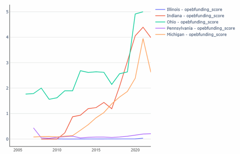
- OPEB Funding Score
- Net Worth Score
- Revenue Growth (Mass Transits Only, Factored into Overall Score)
- Ridership (Mass Transits Only, Not Factored into Overall Score)
- Operating Revenue Percentage (Mass Transits Only, Not Factored into Overall Score)
A challenging part of this research was that the Municipal Finance Database does not provide fiscal strength scores for component units or multistate entities (such as the MTA). Instead, I replicated the calculations used to calculate the fiscal strength scores by collecting data from the Annual Comprehensive Financial Reports (ACFRs) published by the MTA. In addition, I also considered MTA ridership and reliance on transfers when assessing fiscal strength as well.
Illinois: Before and After the MLF Loans
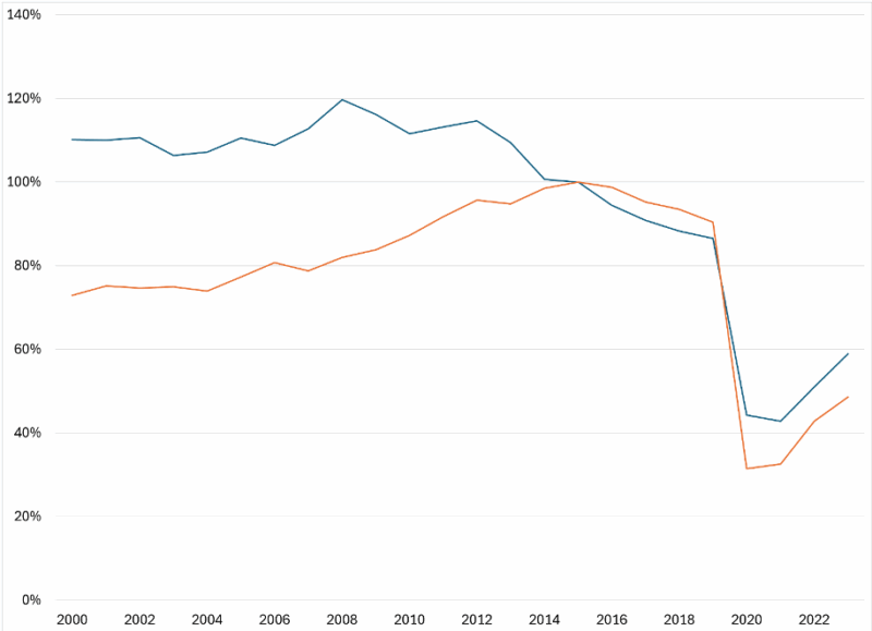
Prior to COVID-19, Illinois was facing severe financial troubles; COVID-19 response and the economic shutdown accelerated the process.[37] Illinois had already been facing a fiscal crisis due to decades of irresponsible fiscal policy, and its credit ratings have been teetering just above junk status since 2017.[38] The Hoover Institution Municipal Finance Dashboard examines state entities with a fiscal strength score based on criteria related to revenue, expenditures, debt, and pension and Other Post Employment Benefits (OPEB).[39] For all years 2006-2022, Illinois ranked among the states with the worst fiscal health. Figure 2 shows the overall fiscal strength of rankings of the State of Illinois, compared to similar states.
Figure 2: Overall Fiscal Strength Score (Out of 100)
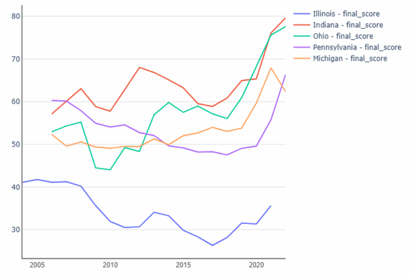
Compared to the other states in this sample, Illinois is relatively weak fiscally. Among all 50 states, Illinois consistently ranks the fiscally weakest from 2006 (first year data for all 50 states are available) through 2021 (the latest available data for Illinois). Only briefly from 2014-2016 does Illinois go from fiscally weakest to second weakest (New Jersey ranked the weakest in those years).
Illinois was the first state to utilize the MLF. In June 2020, Illinois sold $1.2 billion in general obligation bonds to the MLF.[40] Thanks to the MLF, Illinois was able to borrow from the Fed at 3.8 percent, well below the 4.875 percent it would have borrowed at if it sold bonds on the open market in June.[41] In late December 2020, just before the lending facility was set to expire, the MLF purchased an additional $2 billion in general obligation bonds from Illinois, bringing the total loaned to Illinois to $3.2 billion. The Bond Buyer reported that, while the MLF loan was 3.42 percent, if Illinois had sold the bonds on the market, it would have paid a lower interest rate of 3.3 percent. “Despite the high rate,” Yvette Shields of Bond Buyer commented, “market participants have said the state’s decision to use the MLF was a smart move given its market rates fluctuate and its access alone could contribute to improved overall trading levels.”[42] Even at this higher borrowing rate, it is also important to remember that the US Treasury was prepared to fully cover the Fed’s losses if Illinois had not paid the MLF loans back. While those funds helped cover the $6 billion budget deficit, the Fed did not require Illinois to make any structural changes to prevent this from happening again.[43] Illinois did fully pay back the loans.
As of FY 2022, the State of Illinois and its component units owe $58.6 billion in outstanding bonded obligations.[44] Just a year later in FY 2023,[45] its unfunded pension liabilities were $145.552 billion and its unfunded OPEB liabilities were $20.385 billion.[46] In FY 2023, it also reported a net position of -$162 billion.
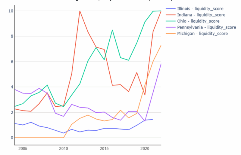
This section will compare Illinois to neighboring Indiana as well as Ohio, Pennsylvania, and Michigan (chosen for similar population size, median household income, and poverty rates). The fiscal strength score measures along ten different variables: reserve position score, debt burden score, liquidity position score, revenue growth score, pension obligation score, pension funding score, pension contribution score, OPEB obligation score, OPEB funding score, and Net Worth Score. The score descriptions and weighting are available in the Appendix.
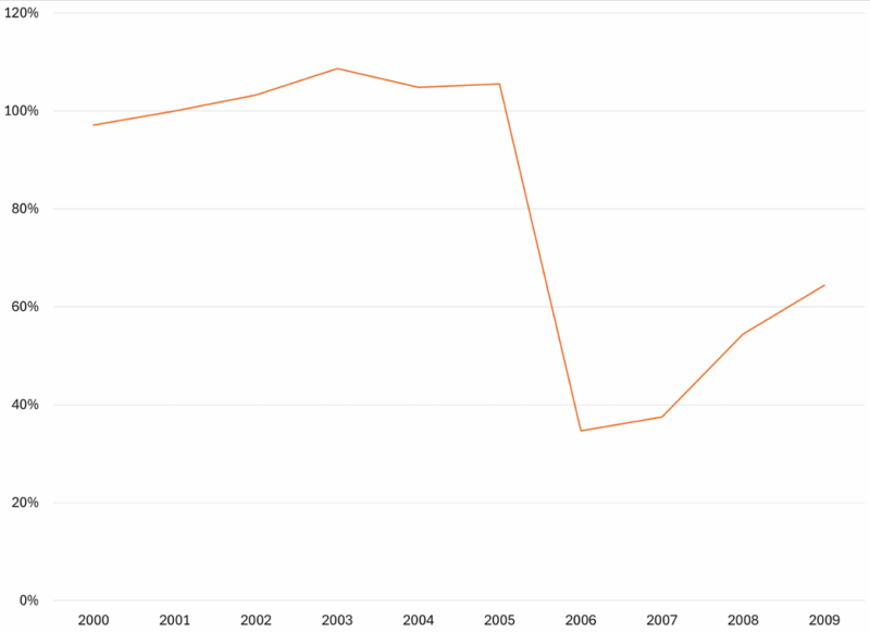
The Reserve Position Score is a variable that measures “how much funds the government has at its disposal to quickly address any liabilities that arise without a renewed appropriation of funds.”[47] This is measured by the average growth rate of unrestricted funds balances over the last three years. The unrestricted fund balance consists of the committed fund balance (amounts that can only be used for specific purposes determined by a formal action of the government’s highest level of decision-making authority), the assigned fund balances (funds that are intended to be used for a specific purpose but do not meet the criteria of being committed or stipulated by law), and unassigned fund balances (the remaining general fund funds not restricted, committed, or assigned).[48] The best scores were able to cover funds for nine months or longer. These results are shown in Figure 3.
Figure 3: Reserve Position Score (Out of 15)
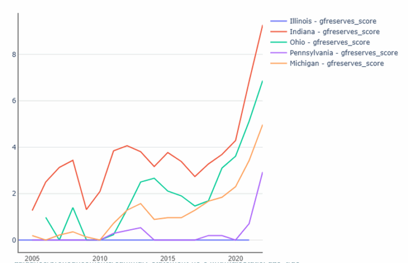
Source: Stanford Municipal Finance Dashboard, “Fiscal Fundamentals: State Comparison”
For all years of available data, Illinois had a Reserve Position Score of zero, although 23 other states also had a score of zero in this category. Although the government holding funds represents an opportunity cost the next highest-valued use to taxpayers had the government not taxed them, the Government Financial Officers Association (GFOA) recommends that all governments maintain an unrestricted fund balance of no less than two months of regular general fund operating revenues or expenditures.[49] Illinois has received a score of 0, but the state government has had a negative net position for all years observed.[50] Thanks to this, Illinois has had to take on billions of dollars in debt to cover budgetary expenses (shown in Figure 4). This weak net position also impacts the state’s liquidity (shown in Figure 5). The liquidity KPI measures the degree to which governments have access to liquid assets to cover any immediate cash outflow. The liquidity KPI measures the liquid assets (general fund cash, cash equivalents, and investments) relative to the fund’s liabilities.
Figure 4: Debt Burden Score (Out of 15)
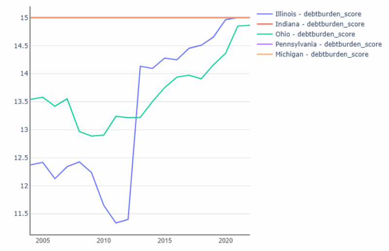
Source: Stanford Municipal Finance Dashboard, “Fiscal Fundamentals: State Comparison”
Figure 4: Debt Burden Score (Out of 15)
Source: Stanford Municipal Finance Dashboard, “Fiscal Fundamentals: State Comparison”
In FY 2019, the year before the pandemic, Illinois and its component units owed $62.3 billion (in nominal dollars) in outstanding bonded obligations. Of that $62.3 billion, $43.5 billion (about 70 percent) of the outstanding debt was in general obligation bonds.[51] This is significant because general obligation bonds are backed by “the full faith and credit of the State of Illinois.”[52] A promise of full faith and credit means that the state promises to use all legally available funds to pay principal and interest owed, and can raise taxes to pay down the debt.[53]
Illinois also amassed billions of dollars in unfunded pension and OPEB liabilities. Illinois is one of three states that protect both public pension and OPEB benefits through the state constitution, which means once a benefit is earned it “shall not be diminished or impaired.”[54] Savidge, et al. (2020) discuss that Illinois has a unique problem of underfunding pension promises. In the white paper, my coauthors and I discuss how Illinois, through state statutes Public Acts 100-0023 and 100-0340, use a formula for contribution calculation that differs from the formula recommended by the Government Accounting Standards Board (GASB). As a result, the state pays a fraction of the required contribution to cover benefits earned that year and to pay down liabilities accrued from previous years.[55] In FY 2019, Illinois pension plans owed $142.4 billion in unfunded liabilities based upon government accounting standards.[56]
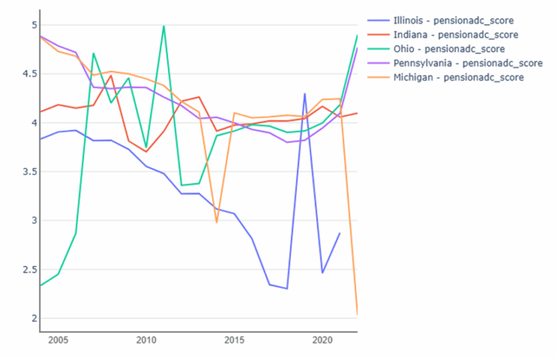
The public pension health scores are shown in Figures 6a (Pension Obligation), 6b (Pension Funding), and 6c (Pension Cost). The spikes in scores following 2020 reflect an increase in transfer payments (via federal pandemic funding) and MLF loans that enabled Illinois to make significant contributions to its public pensions despite an explicit ban from the Treasury for using the funds to cover pension debt.[57]
Figure 6a: Pension Obligation Score (Out of 10)
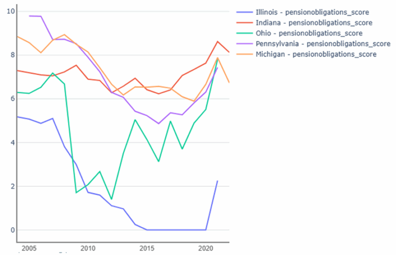
Figure 6b: Pension Funding Score (Out of 5)
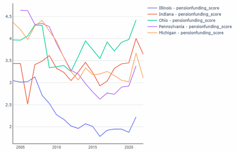
Figure 6c: Pension Contribution Score (Out of 5)
Source: Stanford Municipal Finance Dashboard, “Fiscal Fundamentals: State Comparison”
Also in 2019, Illinois OPEB plans owed $73.5 billion based upon government accounting standards.[58] OPEB plans, such as the Illinois State Employees Group Insurance Program, provide health, dental, vision, and life insurance to retired state and university public employees. The OPEB Health Scores are shown in Figures 7a (OPEB Obligation) and 7b (OPEB Funding). Much like the pension scores of the same name, the obligation score measures the net OPEB obligation (assets minus liabilities) and the funding score measures the funding ratio (assets divided by liabilities expressed as a percentage). OPEB contribution data, however, has limited availability. Under GASB statements 74 and 75, new OPEB accounting standards waived requirements for public OPEB plans to include contribution data. While GASB stated that myriad factors outside of the control of the state government affect OPEB costs (such as changes in healthcare costs and insurance coverage), removing how much states are contributing to OPEB plans leaves public employees and taxpayers in the dark about how well these plans are being funded.[59] Unfortunately, this also obscures how much public employees and taxpayers are being required to set aside each year to cover OPEB expenses.
Figure 7a: OPEB Obligation Score (Out of 10)
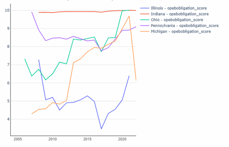
Figure 7b: OPEB Funding Score (Out of 5)
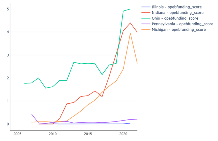
Source: Stanford Municipal Finance Dashboard, “Fiscal Fundamentals: State Comparison”
This massive amount of state debt and unfunded liabilities, accumulated over several decades, did not go unnoticed. Between 2009 and 2017, Moody’s, S&P, and Fitch credit rating agencies downgraded Illinois’ general obligation bond rating 21 times.[60] As of calendar year 2025, Illinois still ranks among the lowest-performing states.
This low performance is reflected in the state net-worth score for Illinois, which is dangerously low for 2002-2014 and then a score of 0 for 2015-2022. Net worth is measured as the unrestricted net position (assets minus liabilities), like a corporate finance definition of net position. Duffy and Giesecke (2024) note that while state governments own “fixed capital assets…most of the capital assets are highly illiquid and thus cannot be used to serve the liabilities.”[61] The Net Worth Score is shown in Figure 8.
Figures 8: Net Worth Score (Out of 15)
Source: Stanford Municipal Finance Dashboard, “Fiscal Fundamentals: State Comparison”
Across every metric and in overall fiscal health, Illinois ranked among the worst-off states and shows little to no sign of improvement. At best, the loans from the MLF helped maintain the pre-2020 status of Illinois. The subsequent data coming out of Illinois is also concerning. As of 2025, Illinois projects a general fund budget deficit of $3 billion starting in 2026, and a budget deficit every year through 2030. By contrast, the state reported a $211 million budget surplus in 2025, showing the rapid deterioration of fiscal health in the absence of support from federal pandemic stimulus packages.[62]
The New York Metropolitan Transportation Authority: The MLF Expands Authority
The Metropolitan Transportation Authority (MTA) is a public benefit corporation providing public transportation for New York City, Long Island, southeastern New York State, and Connecticut.[63] The New York Annual Comprehensive Financial Report (ACFR) lists the financial information of 43 “discretely presented component units” also known as “public benefit corporations,” including the MTA. [64] Being a component unit means that the entity is legally separate from New York State, “managed independently, outside the appropriated budget process, and their powers are generally vested in a governing board…They are not subject to State constitutional restrictions on the incurrence of debt, which apply to the State itself, and may issue bonds and notes within legislatively authorized amounts.”[65] Despite the legal separation, New York State ACFR readily admits that “the State is financially accountable for [these component units] and may be affected by their financial well-being.”[66] Furthermore, the state readily admits that while the Governor of New York does not have authority to appoint members of the governing board, it is a discretely presented component unit because it is fiscally dependent upon, and has a financial benefit or burden relationship with the State…the nature and significance of their relationships with the State are such that it would be misleading to exclude them.”[67]
The relationship between the MTA and New York State, while convoluted, is a clear example of an Off-Budget Enterprise (OBE) as discussed by Bennett and DiLorenzo (1982). An OBE is defined as, “corporations formed by one or more political jurisdictions and are often referred to as authorities, districts, commissions, agencies, and boards.” [68] They write,
“Since one of the major advantages of OBEs to the politician is the creation of patronage opportunities which don’t appear on-budget, the politician has an incentive to subsidize OBEs, if possible, whenever user charges do not cover expenditures or when they are threatened with default.”[69]
Seven years after Bennett and DiLorenzo published their analysis on Off-Budget Enterprises, the Government Accounting Standards Board (GASB) issued “Statement No. 14,” which required state governments to report “discretely presented component units” separately in their financial statements.[70] GASB 14 has since been updated by subsequent statements, most notably GASB 61 in 2010, which expanded reporting requirements, requiring states to present financial information of component units that have “a financial benefit or burden relationship” with the primary government.[71] While GASB reporting requirements have increased transparency into the relationship between New York state and the MTA, the ability to keep MTA and related component units out of the “primary government” budget enables state policymakers to obscure the relationship between the two entities. Despite the greater transparency, Norcross (2010) notes that such “budget gimmickry” encourages governments to “deliberately or inadvertently obscure the cost of policy choices to both policymakers and voters.”[72]
While the Hoover Municipal Finance Dashboard does not provide fiscal strength scores for multistate entities, the dashboard provides a detailed breakdown of the variables used to calculate fiscal strength.[73] I have utilized the publicly available python code to create a fiscal strength score set for the New York MTA (MTA), The Port Authority of New York and New Jersey (PANYNJ), The Chicago Transit Authority (CTA), and the Washington Metropolitan Area Transit Authority (WMATA). Like the MTA, these transit agencies can also be categorized as OBEs. While an outlier, the inclusion of the PANYNJ is used to highlight an entity that was specifically lobbied to be made an eligible issuer of the MLF yet did not access the facility. Importantly, the PANYNJ does not manage its own pension fund and was therefore excluded from the pension score calculations. The fiscal strength scoring rubric for PANYNJ was adjusted accordingly.
In addition to the variables provided, I have also added two additional variables showing the percentage of total revenue made up by operating revenue (which measures the extent that these entities are “self-supporting”), as well as ridership as a percentage of 2015 total annual ridership. These variables, however, are not factored into the overall fiscal strength score.
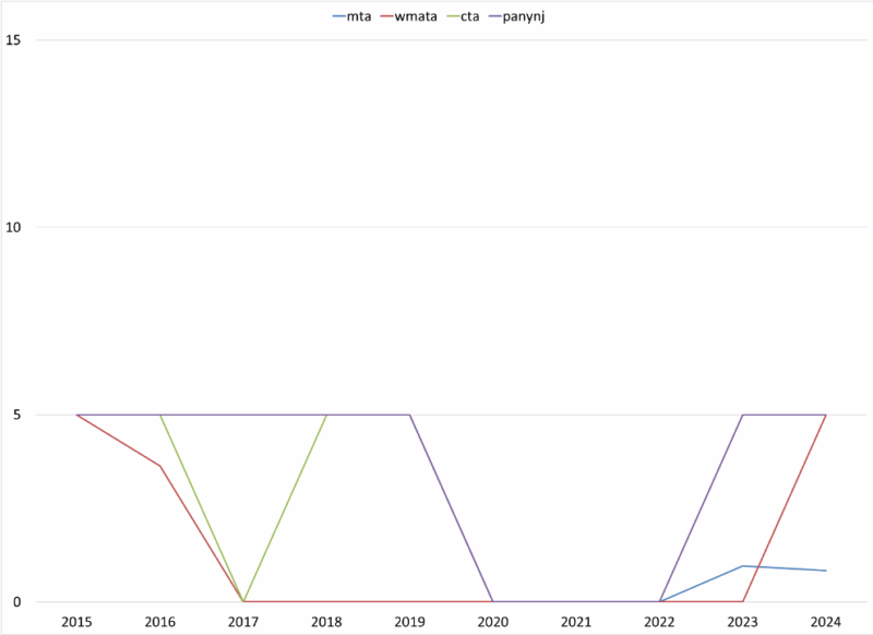
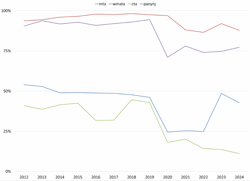
Figure 9: Overall Fiscal Strength Score (Out of 100)
As previously mentioned, the MLF guidelines were amendable at the Federal Reserve’s discretion. This exposed the Federal Reserve and the MLF to political pressure. In April 2020, New York Senator Charles Schumer pressured the Federal Reserve to expand eligible borrowers to multistate entities, such as the Port Authority of New York and New Jersey (PANYNJ).[74] In the end, however, only the MTA took a loan from the Federal Reserve.
This forced expansion of the MLF shows some improvements in fiscal strength in the two years that followed the MLF loan. Initial reports, however, show that the support provided by the MLF and other pandemic-related stimulus packages appear to yield little to no medium- or long-term improvements. In October 2024, New York State Comptroller Thomas DiNapoli noted that the MTA would close the year out with a $211 million deficit that would grow to $652 million by 2028.[75] Other indicators in the Hoover Fiscal Strength Index yield similar results. Overall fiscal strength for all transit systems measured here is dangerously low.
Figure 10: Reserve Position Score (Out of 15)
Sources: Annual Comprehensive Financial Reports of Sampled Mass Transit Systems; Stanford Municipal Finance Dashboard, “Fiscal Fundamentals: State Comparison” and Author’s Calculations.
Despite the injection of funds from pandemic-era stimulus packages as well as the MLF loans, the MTA’s reserve score has remained practically zero (identical to WMATA and the CTA) for all years recorded. The PANYNJ maintains a relatively high reserve score given a positive net position thanks to heavy reliance on user fees and service charges such as leases, landing fees for airports, concessions, and rent from commercial real estate, in addition to tolls and fares.
Figure 11: Debt Burden Score (Out of 15)
Sources: Annual Comprehensive Financial Reports of Sampled Mass Transit Systems; Stanford Municipal Finance Dashboard, “Fiscal Fundamentals: State Comparison” and Author’s Calculations.
Here, we see the debt burden score slightly improve in 2022. As described in the appendix, the debt burden score is calculated by total revenues divided by total long-term debt obligations. In 2021, and 2022, the New York MTA received substantial funding from the American Rescue Plan Act, dramatically increasing total revenues.[76] These transfers also reflect the improvements in MTA scoring in Figures 12-15 during that time, especially when compared with other transit systems.
Figure 12: Liquidity Position Score (Out of 10)
Sources: Annual Comprehensive Financial Reports of Sampled Mass Transit Systems; Stanford Municipal Finance Dashboard, “Fiscal Fundamentals: State Comparison” and Author’s Calculations.
When examining pension scores, the MTA has the strongest scores of the sample. This, however, does not mean the MTA’s pension system is in good financial health. The pension obligation (unfunded liabilities divided by total revenues) shows that revenues could cover promised pension benefits not already covered by prefunded assets, however, fulfilling that obligation would crowd out spending on core MTA services. While the pension funding scores prior to 2020 are above average, the funding ratio used to calculate the score (pension plan assets divided by total liabilities), leaves much to be desired. For context, the American Academy of Actuaries recommends public pension plans have a 100 percent funding ratio. [77] Alternatively, Brainard and Zorn (2012) argue that the 80 percent funding ratio to match private sector plans is sufficient.[78] Using either metric shows the MTA funding ratio to be well below acceptable levels. For all years measured except 2021, the pension funding ratio for the MTA was below 80 percent. The 2021 exception reflects numerous cash transfers received from the federal government. It is again important to note that the PANYNJ does not manage its own pension plan, and thus the lack of pension scores has caused its overall fiscal strength score to be reweighted and rescaled.
Figure 13a: Pension Obligation Score (Out of 10)
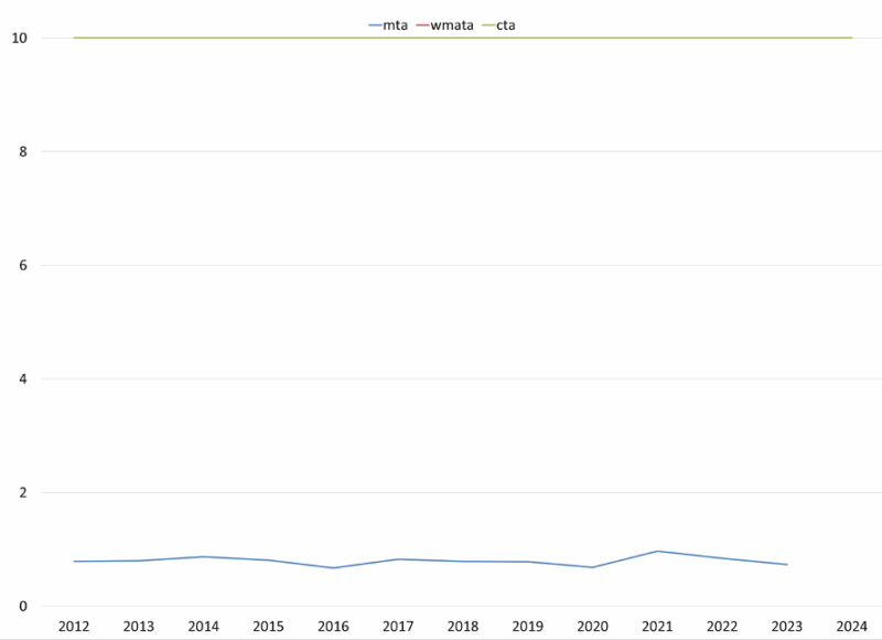
Figure 13b: Pension Funding Score (Out of 5)
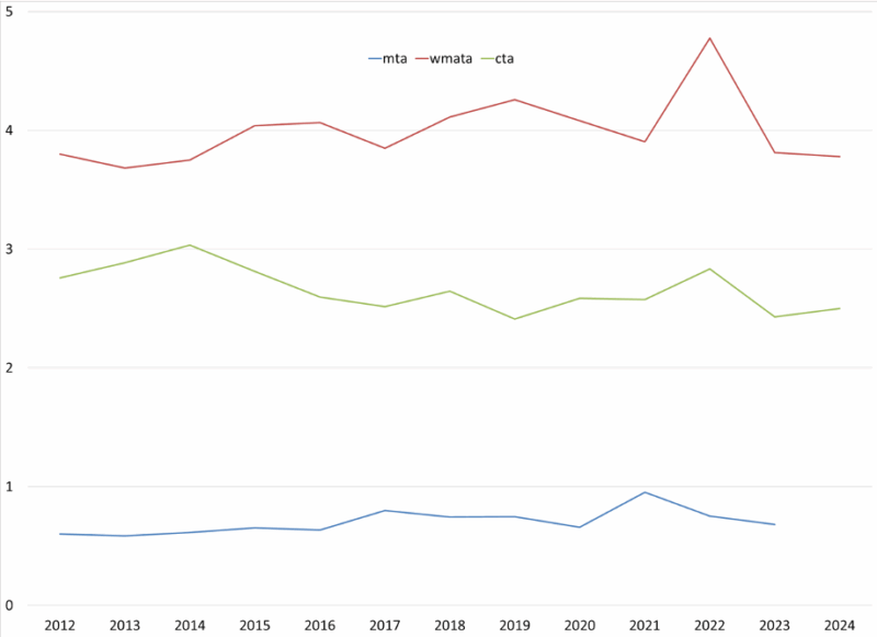
Figure 13c: Pension Contribution Score (Out of 5)
Sources: Annual Comprehensive Financial Reports of Sampled Mass Transit Systems; Stanford Municipal Finance Dashboard, “Fiscal Fundamentals: State Comparison” and Author’s Calculations.
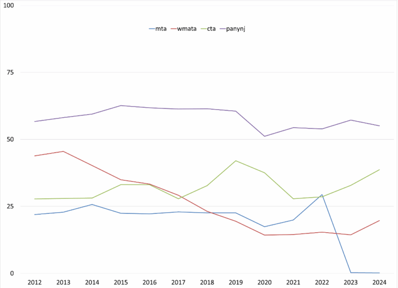
Figure 14a: OPEB Obligation Score (Out of 10)
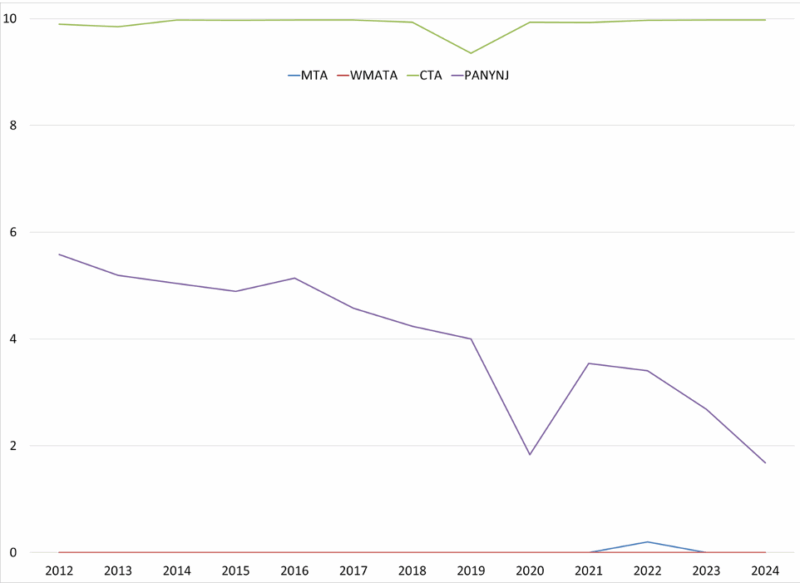
Figure 14b: OPEB Funding Score (Out of 5)
Sources: Annual Comprehensive Financial Reports of Sampled Mass Transit Systems; Stanford Municipal Finance Dashboard, “Fiscal Fundamentals: State Comparison” and Author’s Calculations.
Figure 15: Net Worth Score (Out of 15)
Sources: Annual Comprehensive Financial Reports of Sampled Mass Transit Systems; Stanford Municipal Finance Dashboard, “Fiscal Fundamentals: State Comparison” and Author’s Calculations.
In addition to the scores calculated for state governments, this paper included an additional Revenue Growth KPI Score (provided by Duffy and Giesecke (2024) for the mass transit systems. Duffy and Giesecke (2024) note that revenue growth “how healthy the underlying economy of a given area really is, justifying its use in assessing the financial stability of cities. Loviscek and Crowley (1990) demonstrate that rating agencies frequently use revenue growth as a [bellwether] for the overall health of a given issuer’s economy.”[79] This metric, shown in Figure 16, indicates the health of the economy that these transit systems service. While economic health is impacted by factors outside of the transit system’s influence, it is nonetheless an important indicator of how these transit systems should be managing expenditures.
Figure 16: Revenue Growth Score (Out of 15)
Sources: Annual Comprehensive Financial Reports of Sampled Mass Transit Systems; Stanford Municipal Finance Dashboard, “Fiscal Fundamentals: State Comparison” and Author’s Calculations.
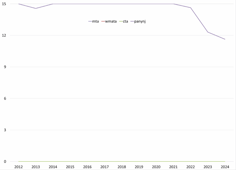
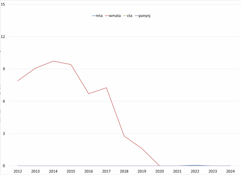
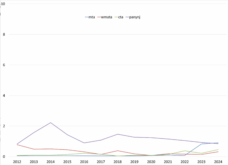
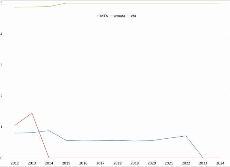
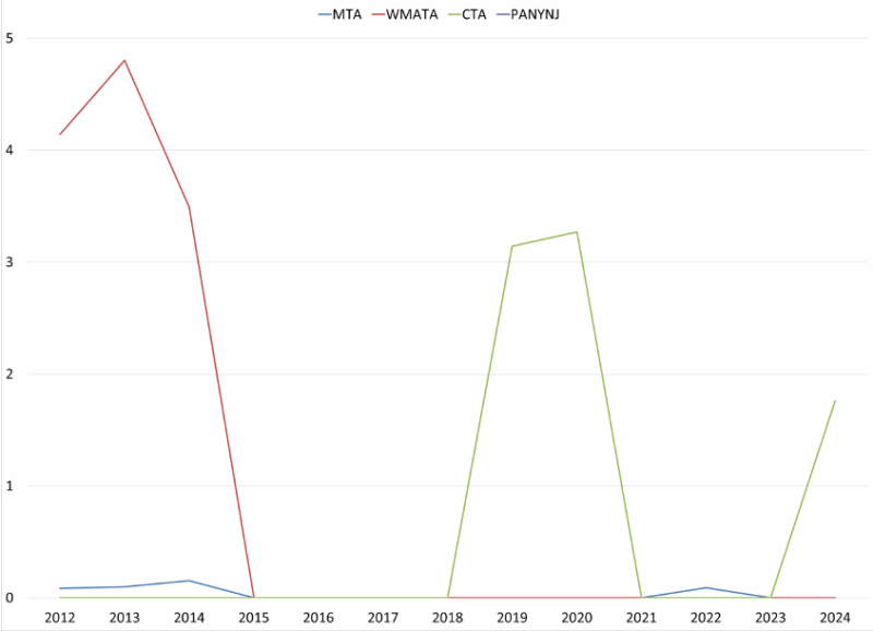
Given the nature of the MTA, it is also important to consider ridership. In the years 2000-2024, ridership across various MTA services peaked in 2015. This year represents a period of stable and robust transit use prior to the subsequent decline starting in 2017 (referred to as the New York City Transit Crisis) which was exacerbated by COVID-19 prevention measures in 2020.[80] Figures 17a-d show ridership as a percentage of 2015 ridership across all transit systems. For the MTA, all but the bridges and tunnels have yet to return to 2015 levels of ridership. Across all transit systems, ridership has yet to return to 2015 levels.
Figure 17a: MTA Ridership as a Percentage of 2015 Ridership
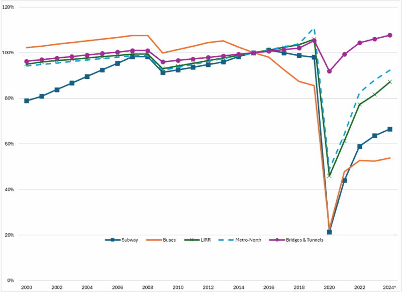
Figure 17b: WAMATA Ridership as a Percentage of 2015 Ridership
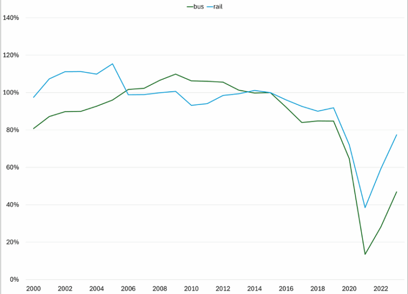
Figures 17c: CTA Ridership as a Percentage of 2015 Ridership
Figures 17d: PATH (PANYNJ) Ridership as a Percentage of 2015 Ridership
Sources: Federal Transit Administration National Transit Databased TS2.1 dataset and Author’s Calculations.Note: 2024 Ridership levels are projected.
Note that ridership and access data are incomplete for PANYNJ. The only available data for PANYNJ concerned the Port Authority Trans-Hudson (PATH) railway.[81] Only estimates for Airport and Port Authority Bus Terminal were available, but these estimates were insufficient and unverifiable. The PATH data reflect similar findings to other rail systems, which have yet to fully recover from the 2020 economic downturn.
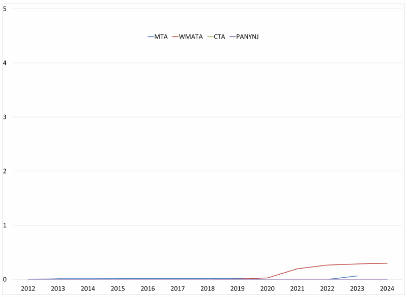
Additionally, it is important to examine the extent to which operating revenue serves as a source of income for these mass transit systems. Operating revenue is the revenue these transit systems receive in the normal course of business (see the Appendix for further information). The less operating revenue available, the more these transit systems are dependent on transfers from federal, state, and local governments as described by Bennett and DiLorenzo (1982). For all years measured, the MTA has the second-lowest operating revenue percentage, indicating a relatively high dependence on governmental transfers and debt financing. Those results are shown in Figure 18.
Figures 18: Operating Revenue Sources as a Percentage of Total Revenue
Sources: Annual Comprehensive Financial Reports of Sampled Mass Transit Systems and Author’s Calculations
Ultimately, the examination of the MTA and related transit shows why, despite Senator Schumer’s pressure for the Fed to accommodate the PANYNJ, the PANYNJ was able to survive without an MLF loan.
The Lasting Impact of the MLF: Bad Behavior Further Enabled
Currently, the Securities Industry and Financial Markets Association (SIFMA) calculates that state, and local governments have a total of $4.1 trillion ($12,312 per person in the US) in outstanding bonded obligations.[82] These obligations, as well as unfunded pension liabilities, continue to grow unabated across the states.
The fiscal strength of Illinois and the MTA do not appear to have improved in the years following the MLF loans. When compared to others in their respective samples, it is difficult to find any noticeable impact of the MLF loans that is distinguishable from the other fiscal programs enacted under the CARES Act or subsequent stimulus packages under the Biden Administration. Perhaps the most damning critique of the MLF loans are the poor liquidity scores for both Illinois and the MTA following 2020, despite the MLF’s explicit goal of providing liquidity to fiscally distressed municipal entities.
The damage of the facility, however, is abundantly clear. The MLF’s creation has generated greater complications for monetary policy. For example, if inflation rises and the Fed wants to tighten policy by raising interest rates, it will face a clear tradeoff: raising interest rates (including the IOR) creates strain on municipal governments, but maintaining low rates to give favorable borrowing rates to municipal entities risks inflation. In addition to pressures from Congress and the President to be more accommodative of federal spending, the Fed is now at risk from rent-seeking state governments as well. Fiscally irresponsible state policymakers will not make necessary budget reforms because they can expect future federal transfers and possibly the Federal Reserve’s below-market-rate loans.
The MLF also creates the potential for policymakers to abuse what Cutsinger and Rouanet (2021) call a “monetary commons.”[83] The money commons, the real value of the money stock, is treated as a common-pool resource. A common-pool resource, as described by Ostrom (1990), “refers to a natural or man-made resource system that is sufficiently large as to make it costly (but not impossible) to exclude potential beneficiaries from obtaining benefits from its use.”[84] Cutsinger and Rouanet (2021) note that the real value of the money stock is a collectively shared resource vulnerable to overuse. Inflation outcomes depend on the political structure governing the monetary authority. In times of political instability, (which are identified as “the result of poorly defined political property rights”) multiple political actors have conflicting claims over the real value of the money stock.[85] Cutsinger and Rouanet write:
“These groups are interdependent but separate in the sense that the members of each group do not belong to other, rival groups. As such, there is nothing attenuating their decision to inflate. When all groups behave this way, the aggregate equilibrium inflation rate that emerges may vastly exceed the seigniorage-maximizing rate, and may lead to a complete abandonment of the currency once the real value of the money stock is dissipated.”[86]
The MLF has now created new rent-seeking groups with claims over the real value of the money stock: state and local governments as well as their related entities. Furthermore, these new groups have an incentive to seek redistributive support from the Fed when in fiscal distress, because successfully receiving said support improves prospects for reelection. As fiscal pressures mount on the Fed to be more accommodating of fiscal policy, its public perception as an “independent agency” will be diluted, which will damage its institutional legitimacy and threaten long-term price stability.[87]
Such rent-seeking groups are likely to appear sooner than expected. As of 2025, both Illinois and the MTA are under new financial stress. In both instances, Illinois and the MTA are hoping for transfer payments to cover budget deficits. Rather than change behavior, policymakers hope that revenue returns to pre-pandemic levels or that the federal government and the Federal Reserve are willing to provide funds when the next budget crisis occurs.
Recommendations for Reform
If fiscal strength is to improve among state and off-budget entities, serious reforms are necessary. This section provides possible reforms at the federal and state level to improve transparency and accountability.
Federal: Ban Bailouts, Update the Bankruptcy Code
The best course of action at the federal level is for policymakers to ex-ante guarantee that the federal government will not use funds to bailout state budgets whether through actions coordinated by the US Treasury or the Federal Reserve.Given that federal taxpayer dollars give federal policymakers influence over state budgets, however, these policymakers have a strong incentive not to issue an ex-ante guarantee, making such a guarantee unlikely.
Alternatively, federal policymakers can create a chapter in the US bankruptcy code for state governments. Under the current US Bankruptcy Code, state governments cannot declare bankruptcy. Legal scholar David Skeel , an American Law Professor who oversaw Puerto Rico’s recent bankruptcy, proposes allowing the states to declare bankruptcy, providing a clear path for a state in danger of default. In turn, the threat of bankruptcy would give state officials leverage to negotiate state obligations outside of bankruptcy, instead of relying on the Contracts Clause to do so.[88],[89]
Economist Veronique de Rugy and legal scholar Todd Zywicki also considered the tradeoffs of allowing states to access the US Bankruptcy Code in the wake of the economic downturn of 2020.[90] They noted that those in favor of creating a bankruptcy code disregarded the problem of rent-seeking groups (such as public employee unions) that could lobby for policy changes in the bankruptcy code that favor the rent-seekers at the expense of the general public. In addition, state bankruptcy could easily backfire. If not done properly, de Rugy and Zywicki warn, bankruptcy will allow states to continue spending patterns that put them in bankruptcy in the first place, restarting the cycle with “a clean slate without providing incentives to change the core source of their financial problems…”[91] David Skeel noted government bankruptcy oversight’s “messiness” in practice.[92] The complexity of restructuring unfunded liabilities and bonded obligations (some of which are still in the process of restructuring) means that bankruptcy is not a “quick fix” to government fiscal woes.[93]
Zywicki and de Rugy also note that opponents to allowing states to access the Bankruptcy Code “tend to make the perfect the enemy of the good.”[94] They also recommend proper constraints such as ensuring bankruptcy negotiations apply to all parties (including bond investors and public employee pensions) and requiring bankruptcy judges be selected at random by the clerk of the court, instead of from the bankruptcy court where the case is located.[95]
While imperfect, allowing states to access the US bankruptcy code (with proper constraints in place) is a preferable alternative to a federal bailout of the state or attempts to declare sovereign immunity.
Federal: Fiscal and Monetary Rules
When looking at the possibility of a balanced budget amendment for the federal government, James Buchanan wrote, “Restoration [of a balanced-budget rule] will require a constitutional rule that will become legally as well as morally binding, a rule that is explicitly written into the constitutional document of the United States.”[96] Recent research has also found that the need for robust balanced-budget requirements are much stronger than when Buchanan first urged them.[97] The most effective balanced budget rules are ones that are constitutionally binding, apply to the entire federal budget, and are permanent. Even strict plans must have some flexibility, such as tying targets or limits to multiyear periods, and carefully constructed emergency provisions (in case of war).[98]
In addition to balanced-budget amendments, the federal government can also apply a “debt brake,” such as the one in Switzerland. In 2001, 85 percent of voters in Switzerland approved an initiative that requires government spending to keep pace with revenue, and limits spending growth to average revenue growth over a multiyear period.[99] The majority of the national budget must be balanced each year and adjusts over the course of the business cycle. This policy is called a “debt brake” because spending must be paid for upfront.[100] The government cannot issue debt to cover budget deficits. This brake does not totally ban the government from issuing debt, but it does slow the growth of debt and shrink the debt. Since its enactment, Swiss Central government debt as a percentage of GDP has declined. From 2020-2021, while the US national debt-to-GDP ratio was growing past 97 percent, the Swiss debt hovered around 20 percent.[101]
This Swiss debt brake, however, owes credit to national tax rates set by the Swiss constitution, which require a double-majority referendum to change. When combined with strong fiscal and monetary rules, a debt brake could feasibly help slow spending growth and debt growth.[102]
Additionally, monetary policy requires serious reforms as well. A return to a gold standard in a decentralized monetary system would offer the best protection against political influence over monetary policy. Cutsinger (2019) shows that, while transitioning back to a gold standard could be feasibly achieved, there are strong political incentives against returning to it.[103]
Absent returning to the gold standard and decentralizing monetary policy, applying constitutional rules to both fiscal and monetary policy offer the best chance at separating the two and enacting fiscal and monetary reforms to each. With respect to a monetary rule, Salter (2021) notes, “a well-designed monetary rule would enable a fiat money regime to outperform the gold standard, provided that the central bank was sufficiently committed to the rule. How to achieve and maintain that kind of a commitment, however, is far from obvious.”[104] Even without a perfect commitment, such a rule would perform better than the current Federal Reserve operating framework, which encourages political influence and mission creep such as the MLF.
Additionally, Cutsinger (2025) offers several politically feasible suggestions to improve the current FAIT system, in addition to a constitutional rule. These include: (1) symmetric inflation targeting, reverting to a stand‑alone 2 percent goal that treats deviations neutrally; (2) symmetric average inflation targeting, which offsets both over‑ and undershoots to stabilize long‑run inflation; (3) raising the inflation target, intended to provide more room for interest‑rate cuts during recessions (though he cautions it offers limited benefits); and (4) nominal GDP (spending) targeting, considered his preferred option, as it aligns with both output and price stability and avoids misinterpreting supply shocks.[105]
State: Fiscal Rules, Control Federal Transfers, and Reform Off-Budget Enterprises
To avoid fiscal crises, state policymakers must also make reforms to state spending, including state relationships with federal programs and off-budget enterprises.
Primarily, improvements to state fiscal policy must be made through tax and expenditure limits (TELs). This kind of a spending limit provides fiscal discipline during periods of strong revenue growth, while avoiding overspending and the creation of structural deficits. This two-pronged policy makes state budgets more resilient in the face of unanticipated expenses. When properly designed and implemented, tax and expenditure limitations can be effective in constraining the growth of government spending and stabilizing budgets over the business cycle.
Such a policy has been in effect in Colorado since 1992: The Taxpayer’s Bill of Rights (TABOR) amendment to the Colorado Constitution.[106] TABOR has revenue and expenditure limitations that apply to state and local governments. The revenue limitation applies to all tax revenue, prevents new taxes and fees, and can only be overridden by popular vote. Expenditures are limited to revenue from the previous year, plus the rate of population growth, plus inflation. Any revenue above this limitation must be refunded, with interest, to Colorado citizens.
TELs are much more effective when incorporated into state constitutions rather than into statutes, more easily evaded or ignored. The most effective TELs also limit the rate of growth of revenue and expenditures to the sum of inflation plus population growth. If states link TELs to a measure of aggregate economic activity, like personal income, it will be less effective in stabilizing the budget, because personal income is a more volatile measurement than the sum of population and inflation growth.[107] In the end, like any other constitutional constraint, a TEL is most effective when it applies to the entire budget.
After tackling their own spending, state and local policymakers must take preemptive actions to limit their dependence on federal transfers. The first step would be to track how much federal money is coming into state and local budgets and the specific areas of government funded by federal dollars. Once federal funds are accounted for, state legislatures can require state agencies to have an emergency plan in place in case of a 5 to 25 percent cut in funding (simulating a cut in federal funds) and require state agencies to seek legislative approval before applying to federal grant programs. These strategies have been largely successful for Utah as part of its “Financial Ready Utah” plan, enacted in the wake of the Great Recession.[108]
Finally, states must reform their relationships with off-budget enterprises (OBEs), such as the New York MTA. As previously discussed, while changes in GASB rules provided greater transparency over the relationship between state governments and OBEs, these entities still enjoy operating outside of most state fiscal constraints. To this end, OBEs must be brought fully on budget — subject to the same fiscal constraints as official public entities — or must be taken off-budget entirely.
Prospects for Reform
Despite the Federal Reserve’s intervention in the municipal bond market in 2020, fiscal strength improvements (particularly liquidity improvements) for the lending entities were barely distinguishable from their relative samples. The damage from the MLF’s creation is apparent. Monetary officials continue to embrace mission creep while fiscal policymakers are free to pressure the Fed to accommodate fiscal policy. In short, the facility enabled the bad behavior of all parties involved.
The federal government must make an explicit commitment not to bail out state government budgets or their related entities.
With the risk of future Fed interventions into the municipal bond market and increased probability of a federal bailout of the states, it is safe to concur with Cachanosky et al. 2021’s conclusion that the creation of the MLF was “unwarranted and unwise.”[109]
Appendix-Stanford Municipal Finance Fiscal Indicators
The following methodological discussion is taken directly from the “Hoover Institution Municipal Finance Issuer Fundamentals” (with some changes in the variable names and description for greater clarity). [110] This measurement utilizes Duffy and Giesecke (2024) “State and Local Government Financial Fundamentals”.[111] Source code for this paper and the Stanford Dashboard are available upon request. Additionally, the code that implements the weighting and re-scaling of Overall Fiscal Strength is available upon request. The Overall Fiscal Strength score is broken down into several Key Performance Indicators (KPI).
Additionally, some changes were made for the mass transit systems. I replaced “general fund revenues” with “operating revenues” and government-wide revenues with “total revenues.” I also used the net position in place of general fund reserves,
Overall Fiscal Strength Score – The fiscal strength of a government consists of many diverse aspects, including debt burden, liquidity position, and pension and OPEB obligations. The overall fiscal strength score aggregates 10 dimensions of financial strength into a single score that ranges from 0 (worst) to 100 (best). It provides a summary of the overall fiscal standing. The scores are weighted at two levels: First Duffy and Giesecke assign a weight at the category level as tabulated in the left column of Table 1. Second, they assign a weight at the score level as tabulated in the right column of the table. Further details about weighting can be found in Duffy and Giesecke (2024).
Weights, by Category and Score
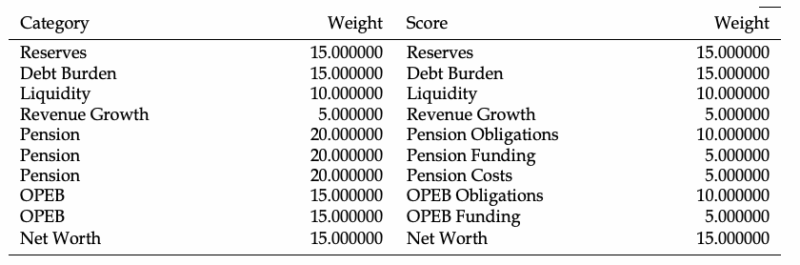
Sources: Duffy, Seamus and Giesecke, Oliver, “State and Local Government Financial Fundamentals.” 7 Sept 2023 (revised 3 Apr 2024). Accessed 30 October 2024 Available at SSRN: https://ssrn.com/abstract=4565350 or http://dx.doi.org/10.2139/ssrn.4565350
Reserve Position Score – The reserve position score rates the extent to which a state or local government’s general fund reserves are sufficient to cover general fund expenditures. This is calculated as follows:

Debt Burden Score – The debt burden score rates the size of the government’s long-term obligations (excluding pension, OPEB) relative to the revenues of the government. This is calculated as follows:

Liquidity Position Score – The liquidity position score rates the extent to which general fund cash, cash equivalents, and investments will cover the general fund’s liabilities. This is calculated as follows:

Revenue Growth Score – The revenue growth score rates the growth of general fund revenue over the last 3 years. This is calculated as follows:
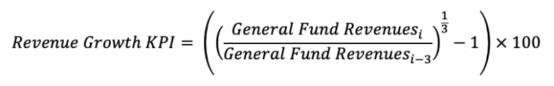
Where “i” represents the year.
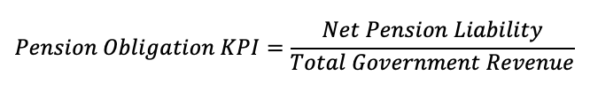
Pension Obligation Score – The pension obligation score rates the size of a government’s net pension liabilities (promised benefits not covered by pension assets, also known as unfunded pension liabilities)[112] relative to the government-wide revenue. This is calculated as follows:
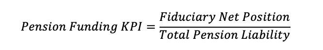
Pension Funding Score – The pension funding score rates the degree to which a government fully funds its pension liabilities. This is measured as the pension funding ratio, which calculates the total pre-funded assets (fiduciary net position) divided by the total promised benefits (total pension liability). This is calculated as follows:
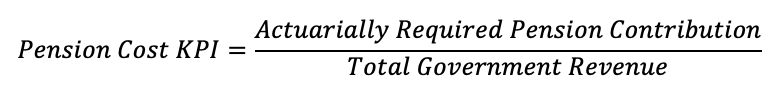
Pension Contribution Score – The pension contribution score rates the size of a pension system’s actuarially required contributions relative to government-wide revenues. The actuarially required contribution is the amount actuarially calculated each year that is required to be contributed by taxpayers to a pension plan asset pool in order to cover benefits accrued in the current year (normal costs) and promised benefits accrued in previous years not covered by pension assets (unfunded liabilities).[113] This is calculated as follows:
OPEB Obligation Score – OPEB (Other Post-Employment Benefit) is a benefit provided to a retired public employee that does not qualify as a pension. These benefits include retiree health insurance, prescription drug plans, and Medicare supplement plans.[114] The OPEB obligation score rates the size of a government’s net OPEB liabilities relative to the government-wide revenue. This is calculated as follows:

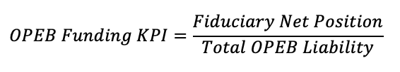
OPEB Funding Score – The OPEB funding score rates the degree to which a government fully funds its OPEB liabilities. It is measured as a funding ratio like that of a pension funding ratio, which calculates the total pre-funded assets (fiduciary net position) divided by the total promised benefits (total OPEB liability).[115] This is calculated as follows:
Note that OPEB Contributions are not scored because OPEB contribution data are no longer required by government accounting standards, leading to serious gaps in contribution data.[116] The reason cited by government accounting standards was that OPEB contributions are determined by exogenous factors such as healthcare cost trends and mortality rates, in addition to the normal cost and unfunded liability components used to determine pension benefits.[117]
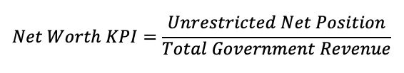
Net Worth Score – The net worth score rates the size of a government’s unrestricted net position (government assets minus government liabilities) relative to the government-wide revenues. Duffy and Giesecke (2024) comment,
“The use of the unrestricted net position derives its justification under the premise that most of the capital assets are highly illiquid and thus cannot be used to serve the liabilities. Giesecke, Mateen, and Sena (2022)[118] show that the unrestricted net position over revenues is strongly correlated with the borrowing cost in the municipal bond market. Several studies have used the unrestricted net position in their measurement of the overall financial stability of the government in question (Clark and Gorina, 2017[119]; Gorina, Joffe, and Maher, 2018[120]; Gerrish and Spreen, 2017[121]).”[122]
This is calculated as follows:
Variables added by the author not included in the Fiscal Strength Scoring Calculation for Mass Transit Systems
Operating Revenue Percentage– This variable measures the percentage of operating revenues to total revenue for a mass transit system. Operating revenues are revenues received during regular business (i.e. farebox and toll revenues, airport fees, and revenue from property rentals and leases) but do not include dedicated taxes or transfers from the government. This measurement serves as a means of determining the extent to which a mass transit system is “self-supporting.” This is calculated for any given year as:
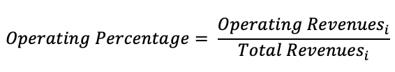
Where “i” represents the year.[123]
Ridership as a Percentage of 2015 Ridership – This variable measures the percentage of 2015 ridership. Among the mass transit systems surveyed, 2015 appears to be a peak year among post-2008 and pre-2020 ridership. Examining annual ridership as a percentage of 2015 ridership is used to control for size differences among these transit systems. Unfortunately, the Port Authority of New York and New Jersey has limited data available for its ridership and access, so the Port Authority Trans-Hudson (PATH) heavy rail rapid transit system. This is calculated as:
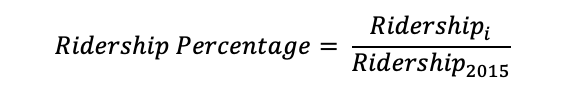
Where “i” represents the year.
End Notes
[1] Cachanosky, Nicolas; Cutsinger, Bryan; Hogan, Thomas; Luther, William; and Salter, Alexander. “The Federal Reserve’s Response to the COVID-19 Contraction: An Initial Appraisal.” Southern Economic Journal, Vol. 87 (4) 2021: 1152-1174 (AIER Sound Money Project Working Paper No. 2021-01). Revised 27 Jun 2022 (posted 9 Nov 2020). https://ssrn.com/abstract=3726345 or http://dx.doi.org/10.2139/ssrn.3726345
[2] Ibid.
[3] Buchanan, James M. Public Principles of Public Debt. The Collected Works of James M. Buchanan Vol. 2 of 20. Indianapolis: Liberty Fund. Available online: https://oll.libertyfund.org/titles/brennan-the-collected-works-of-james-m-buchanan-vol-2-public-principles-of-public-debt
[4] Yonk, Ryan and Savidge, Thomas. Understanding Public Debt. American Institute for Economic Research. 20 August 2024. Accessed September 27, 2024. https://www.aier.org/article/understanding-public-debt/
[5] Henderson, David R. “Present Value” in the Concise Encyclopedia of Economics on Econlib. Retrieved May 6, 2024. https://www.econlib.org/library/Enc/PresentValue.html
[6] For a thorough discussion of discounting public pension liabilities see: Novy-Marx, Robert, and Joshua D. Rauh. 2009. “The Liabilities and Risks of State-Sponsored Pension Plans.” Journal of Economic Perspectives, 23 (4): 191–210. https://www.aeaweb.org/articles?id=10.1257/jep.23.4.191
[7] Savidge, Thomas, Williams, Jonathan, and Estes, Skip. State Bonded Obligations, 2019. American Legislative Exchange Council. 3 Feb 2020. Accessed September 27, 2024. https://alec.org/publication/state-bonded-obligations-2019/
[8] Savidge, Thomas, Williams, Jonathan, and Stark, Nicholas. Other Post-Employment Benefit Liabilities, 5th Edition. American Legislative Exchange Council. 7 Jul 2022. Accessed October 29, 2024. https://alec.org/publication/other-post-employment-benefit-liabilities-5th-edition/
[9] Savidge, Thomas, Williams, Jonathan, and Estes, Skip. Unaccountable and Unaffordable, 2020. American Legislative Exchange Council. 24 Jun 2021. Accessed September 27, 2024. https://alec.org/publication/unaccountable-and-unaffordable-2020/
[10] “Federal Grants to State and Local Governments: A Historical Perspective on Contemporary Issues (R40638).” Congressional Research Service. Updated 22 May 2019. Accessed September 5, 2024. https://www.everycrsreport.com/reports/R40638.html
[11] Ibid.
[12] Ibid.
[13] Ibid.
[14] “State Expenditure Report 2023.” National Association of State Budget Officers (NASBO). Accessed September 9, 2024. https://www.nasbo.org/reports-data/state-expenditure-report
[15] Hamburger, Philip. Purchasing Submission: Conditions, Power, and Freedom. Harvard University Press, 2021. https://www.hup.harvard.edu/books/9780674258235.
[16] Luther, William J. “How Does the Fed Influence the Federal Funds Rate in a Corridor System?” American Institute for Economic Research, June 25, 2018, https://www.aier.org/article/how-does-the-fed-influence-the-federal-funds-rate-in-a-corridor-system/.
[17] Luther, William J. “How Does the Fed Influence the Federal Funds Rate in a Floor System?” American Institute for Economic Research, June 25, 2018, https://www.aier.org/article/how-does-the-fed-influence-the-federal-funds-rate-in-a-floor-system/.
[18] Selgin, George. The Menace of Fiscal QE. Washington, DC: Cato Institute, 2020.
[19] Ibid.
[20] Plosser, Charles I. “Fiscal Policy and Monetary Policy: Restoring the Boundaries” at the U.S. Monetary Policy Forum. The Initiative on Global Markets from University of Chicago Booth School of Business. February 24, 2012. https://www.philadelphiafed.org/the-economy/monetary-policy/speech-archive-president-plosser#2012
[21] “George Selgin on Average Inflation Targeting and The Menace of Fiscal QE,” Macro Musings Podcast, Mercatus Center, September 7, 2020,” Accessed 19 July 2025. https://www.mercatus.org/macro-musings/george-selgin-average-inflation-targeting-and-menace-fiscal-qe
[22] Cutsinger, Bryan P. Rethinking the Fed’s Framework: Lessons from the Post-Pandemic Inflation, AIER White Paper #10 (Great Barrington, MA: American Institute for Economic Research, 2025), https://aier.org/article/rethinking-the-feds-framework-lessons-from-the-post-pandemic-inflation/#executive-summary
[23] Rouanet, Louis and Salter, Alexander William, Mission creep at the Federal Reserve (July 14, 2024). AIER Sound Money Project Working Paper No. 2024-09, Southern Economic Journal, forthcoming, Available at SSRN: https://ssrn.com/abstract=4598286 or http://dx.doi.org/10.2139/ssrn.4598286
[24] “Term Sheet of the Municipal Liquidity Facility (June 3, 2020).” Board of Governors of the Federal Reserve System. 3 June 2020. https://www.federalreserve.gov/monetarypolicy/muni.htm
[25] Ibid.
[26] Haughwout, Andrew, Hyman, Ben, and Shachar, Or. “The Municipal Liquidity Facility.” Federal Reserve Bank of New York Economic Policy Review. Vol. 28, No.1 (June 2022). Accessed January 2025. https://www.newyorkfed.org/medialibrary/media/research/epr/2022/epr_2022_mlf_haughwout.pdf
[27] Term Sheet of the MLF, supra note 38.
[28] Ibid.
[29] “COVID-19: The Federal Reserve’s Municipal Liquidity Facility.” Congressional Research Service. 14 Aug 2020. Accessed October 21, 2024. https://crsreports.congress.gov/product/pdf/IF/IF11621
[30] Joffe, Marc. “Will the Fed kill the municipal bond market?” The Bond Buyer. 29 June 2020. Retrieved from: https://www.bondbuyer.com/opinion/will-the-fed-kill-the-municipal-bond-market
[31] Ibid.
[32] Boettke, Peter; Salter, Alexander William; and Smith, Daniel J. Money and the Rule of Law: Generality and Predictability in Monetary Institutions. Cambridge: Cambridge University Press (2021). p. 99.
[33] Ibid.
[34] Ibid.
[35] “Appendix B: Municipal Liquidity Facility—Pricing Appendix.” Federal Reserve Bank of New York. April 2020. Accessed October 21, 2024. https://www.newyorkfed.org/medialibrary/media/markets/municipal-liquidity-facility-pricing
[36] “Municipal Liquidity Facility Sample Purchase Rates.” Federal Reserve Bank of New York. 3 August 2020. https://www.newyorkfed.org/markets/municipal-liquidity-facility/municipal-liquidity-facility-sample-rates
[37] Savidge, Thomas. “Lockdowns Accelerate Fiscal Crisis in Illinois.” American Legislative Exchange Council. 2 July 2020. https://www.alec.org/article/lockdowns-bring-the-long-run-to-illinois-sooner-than-expected/
[38] Savidge, Thomas. “In Illinois, Reckless Fiscal Policy Colliding with COVID-19.” American Legislative Exchange Council. 10 April 2020. https://www.alec.org/article/in-illinois-reckless-fiscal-policy-colliding-with-covid-19/
[39] Other Post Employment Benefits (OPEB) are guaranteed retirement benefits other than an employee’s monthly pension check. This includes retiree health insurance, Medicare supplement plans, prescription drug plans, disability, and life insurance.
[40] Dabrowski, Ted. “Mismanaged Illinois become first state to borrow from new Federal Reserve facility” Wirepoints. 4 June 2020. https://wirepoints.org/mismanaged-illinois-becomes-first-state-to-borrow-from-new-fed-reserve-facility-wirepoints/
[41] Joffe, Marc. “Will the Fed kill the municipal bond market?” The Bond Buyer. 29 June 2020. Retrieved from: https://www.bondbuyer.com/opinion/will-the-fed-kill-the-municipal-bond-market
[42] Shields, Yvette. “Illinois pockets $2 billion Fed Municipal Liquidity Facility loan” The Bond Buyer. 18 Dec 2020. Accessed October 21, 2024. https://www.bondbuyer.com/news/illinois-pockets-2b-fed-mlf-loan
[43] Schuster, Adam. “S&P: Illinois Faces Junk Rating, Large Budget Deficit Even With Progressive Tax Revenue.” Illinois Policy Institute. 8 October 2020. Retrieved from: https://www.illinoispolicy.org/sp-illinois-faces-junk-rating-large-budget-deficit-even-with-progressive-tax-revenue/
[44] Savidge, Thomas, Williams, Jonathan, Meyer, Joshua. State Bonded Obligations, 5th Edition. American Legislative Exchange Council. Forthcoming.
[45] As of May 2025, the State of Illinois has only released an Interim Report and not a full Annual Comprehensive Financial Report. That means that these initial figures listed for FY 2023 are unaudited and may be subject to change.
[46] “Fiscal Year 2023: Interim Report” Illinois State Comptroller. Accessed October 20, 2024. https://illinoiscomptroller.gov/financial-reports-data/find-a-report/comprehensive-reporting/annual-comprehensive-financial-report/
[47] Duffy, Seamus and Giesecke, Oliver, “State and Local Government Financial Fundamentals.” 7 Sept 2023 (revised 3 Apr 2024). Accessed 30 October 2024 Available at SSRN: https://ssrn.com/abstract=4565350 or http://dx.doi.org/10.2139/ssrn.4565350
[48] “Summary of Statement No. 54.” Government Accounting Standards Board (GASB). Feb 2009. Accessed October 30, 2024. https://gasb.org/page/pronouncement?pageId=/standards-and-guidance/pronouncements/summary-statement-no-54.html&isStaticPage=true
[49] “Best Practices: Fund Balance Guidelines for the General Fund.” Government Financial Officers Association (GFOA). Accessed October 30, 2024. https://www.gfoa.org/materials/fund-balance-guidelines-for-the-general-fund#anchor2
[50] “Annual Comprehensive Financial Reports (multiple years).” Office of the Illinois State Comptroller. Accessed October 30, 2024. https://illinoiscomptroller.gov/financial-reports-data/find-a-report/comprehensive-reporting/annual-comprehensive-financial-report/
[51] Savidge, Thomas, Williams, Jonathan, and Estes, Skip. State Bonded Obligations, 2019. American Legislative Exchange Council. 11 Feb 2020. Accessed October 10, 2024. https://alec.org/publication/state-bonded-obligations-2019/
[52] 30 ILCS 330: General Obligation Bond Act. Illinois Complied Statutes. Illinois General Assembly. Accessed October 10, 2024. https://www.ilga.gov/legislation/ilcs/ilcs3.asp?ActID=508&ChapterID=7
[53] Glossary of Municipal Security Terms (Third Edition). Municipal Securities Ratings Board (MSRB). August 2013. Retrieved from: http://www.msrb. org/msrb1/pdfs/MSRB-Glossary-of-Municipal-Securities-Terms-Third%20Edition-August-2013.pdf
[54] Illinois State Constitution, Article XIII, Section 5.
[55] Savidge, Thomas, Williams, Jonathan, and Estes, Skip. Unaccountable and Unaffordable, 2019. American Legislative Exchange Council. 9 Jun 2020. Accessed October 10, 2024. https://alec.org/publication/unaccountable-and-unaffordable-2019/
[56] Ibid.
[57] Veuger, Stan; Clemens, Jeffrey; Giesecke, Oliver; and Rauh, Joshua. “What Do States Do with Fiscal Windfalls? Evidence from the Pandemic.” American Enterprise Institute Policy Working Paper Series. 28 Feb 2024. Accessed 24 Jun 2024. https://www.aei.org/research-products/working-paper/what-do-states-do-with-fiscal-windfalls-evidence-from-the-pandemic/
[58] Savidge, Thomas and Williams, Jonathan. Other Post-Employment Benefit Liabilities, 6th Edition. American Legislative Exchange Council. 1 Feb 2024. Accessed October 11, 2024. https://alec.org/publication/other-post-employment-benefit-liabilities-6th-edition/
[59] Savidge, et al. Other Post-Employment Benefits, 5th Edition. Supra note 8.
[60] “Illinois Moves Closer to Becoming First ‘Junk’ State With Negative Credit Outlook.” Illinois Policy Institute. 12 Apr 2020. Accessed October 11, 2024. https://www.illinoispolicy.org/illinois-moves-closer-to-becoming-first-junk-state-with-negative-credit-outlook/
[61] Duffy and Giesecke (2024). Supra note 45.
[62] Mishra, Ravi, and Lauren Zuar. Illinois Forward 2026: How the State Can Spend Responsibly. Chicago: Illinois Policy Institute, February 12, 2025. https://www.illinoispolicy.org/reports/illinois-forward-2026-how-the-state-can-spend-responsibly/.
[63] “The Reporting Entity.” Metropolitan Transportation Authority Annual Comprehensive Financial Report for the Years Ended December 31, 2023, and 2022. Accessed October 25, 2024. P.7 https://new.mta.info/investor-info/disclosure-filings
[64] “The Statement of Net Position and the Statement of Activities.” New York State Annual Comprehensive Financial Report for the Fiscal Year Ended March 31, 2024. Accessed October 25, 2024. P. 168. https://www.osc.ny.gov/reports/finance
[65] Ibid.
[66] Ibid. P. 23.
[67] Ibid. p. 168.
[68] Bennett, James T. and DiLorenzo, Thomas J. “Off-budget activities of local government: The bane of the tax revolt.” Public Choice. Vol 39 p. 333-342 (1982). Accessed October 25, 2024. P. 334 https://link.springer.com/article/10.1007/BF00118791
[69] Ibid.
[70] “Summary of Statement No. 14.” Government Accounting Standards Board (GASB). June 1991. Accessed October 25, 2024. https://gasb.org/page/PageContent?pageId=/standards-and-guidance/pronouncements/summary-statement-no-14.html
[71] Summary of Statement No. 91.” Government Accounting Standards Board (GASB). Nov 2010. Accessed October 25, 2024. https://gasb.org/page/pronouncement?pageId=/standards-and-guidance/pronouncements/summary-statement-no-61.html&isStaticPage=true
[72] Norcross, Eileen, Fiscal Evasion in State Budgeting (July 2010). Mercatus Working Paper, No. 10-39, Available at SSRN: https://ssrn.com/abstract=3245331 or http://dx.doi.org/10.2139/ssrn.3245331
[73] Duffy and Giesecke (2024). Supra note 45.
[74] “Press Release: After Schumer Push, Port Authority now has unprecedented and immediate access to hundreds of billions in capital dollars…can now directly access the Federal Reserve’s new lending facility.” Office of Senator Charles E. Schumer. 29 April 2020. https://www.schumer.senate.gov/newsroom/press-releases/after-schumer-push-port-authority-now-has-unprecedented-and-immediate-access-to-hundreds-of-billions-in-capital-dollars-that-can-be-used-to-sustain-critical-projects_needs-including-revamp-of-ny-airports-pa-can-now-directly-access-the-federal-reserves-new-lending-facility
[75] DiNapoli, Thomas P. DiNapoli: MTA Budget Gaps Return. Albany: Office of the New York State Comptroller, October 23, 2024. https://www.osc.ny.gov/press/releases/2024/10/dinapoli-mta-budget-gaps-return.
[76] Metropolitan Transportation Authority. “Federal Funding Provides MTA with Financial Stability Through First Half of 2024; No Fare Increase in 2021.” Press release. July 21, 2021. https://www.mta.info/press-release/federal-funding-provides-mta-financial-stability-through-first-half-of-2024-no-fare.
[77] American Academy of Actuaries. The 80 Percent Pension Funding Myth. Washington, DC: American Academy of Actuaries, April 3, 2014. https://actuary.org/publication-issue/the-80-pension-funding-myth/.
[78] Keith Brainard and Paul Zorn, The 80 Percent Pension Funding Threshold: Its Source as a Healthy or Minimum Funding Level for Public Pension Plans (Washington, DC: National Association of State Retirement Administrators, January 2012), https://www.nasra.org/files/Topical%20Reports/Funding%20Policies/80_percent_funding_threshold.pdf
[79] Duffy and Giesecke, 2024, supra note 45, p.9.
[80] The “New York City Transit Crisis” beginning in 2017 occurred as numerous MTA services (especially the NYC Subway System) suffered from declining revenue, signal slowdowns, and degrading infrastructure. For a brief summary and subsequent issues after 2020, see: Stephen Nessen and Ramsey Khalifeh, “A State of Collapse: How the MTA Put Riders on the Fast Track to Ruin,” Gothamist, January 13, 2025, https://gothamist.com/news/a-state-of-collapse-how-the-mta-put-riders-on-the-fast-track-to-ruin.
[81] Federal Transit Administration. 2023 TS2.1 – Service Data and Operating Expenses Time Series by Mode. National Transit Database, 2024. https://www.transit.dot.gov/ntd/data-product/ts21-service-data-and-operating-expenses-time-series-mode.
[82] “US Municipal Bond Statistics” Securities Industry and Financial Markets Association (SIFMA). Updated 12 September 2024. Accessed September 27, 2024. https://www.sifma.org/resources/research/us-municipal-bonds-statistics/
[83] Cutsinger, Bryan, and Rouanet, Louis. “Democracy, Dictatorship, and the Monetary Commons”. Free Market Institute Research Paper No. 3934048. SSRN, October 1, 2021. http://dx.doi.org/10.2139/ssrn.3934048.
[84] Ostrom, Elinor. Governing the Commons: The Evolution of Institutions for Collective Action. Cambridge: Cambridge University Press (1990). P. 30.
[85] Cutsinger and Rouanet (2021), supra note 79.
[86] Ibid.
[87] [85] For further discussion of the MLF, moral hazard, and a tragedy of the monetary commons, see Cooper, Nicholas K. Essays on the Political Economy of Central Banking. Dissertation defense. Advised by Lawrence H. White. Department of Economics, George Mason University. July 6, 2023. https://economics.gmu.edu/defenses/1485
[88] The US Contracts Clause (Article I, Section 10, Clause 1 of the U.S. Constitution) says that no state can enact a law “impairing” contractual obligation.
[89] Skeel, David. “State Bankruptcy Revisited.” National Affairs. Summer 2020. Accessed March 8, 2024. https://nationalaffairs.com/publications/detail/state-bankruptcy-revisted
[90] de Rugy, Veronique and Zywicki, Todd. “The Difficult Path to State Bankruptcy” The Mercatus Center at George Mason University. 11 June 2020. Accessed March 8, 2024. https://www.mercatus.org/research/policy-briefs/difficult-path-state-bankruptcy
[91] Ibid.
[92] Skeel, David, “State Bankruptcy Revisited.” National Affairs. Vol 56 (Summer 2020). https://nationalaffairs.com/publications/detail/state-bankruptcy-revisted
[93] “Puerto Rico’s Debt Restructuring Process” The Puerto Rico Oversight, Management, and Economic Stability Board. Accessed July 22, 2024. https://oversightboard.pr.gov/debt/
[94] de Rugy and Zywicki, supra note 104.
[95] Ibid.
[96] Buchanan, James, and Richard Wagner. Democracy in Deficit: The Political Legacy of Lord Keynes. Indianapolis: Liberty Fund, 1977. https://oll.libertyfund.org/titles/wagner-democracy-in-deficit-the-political-legacy-of-lord-keynes.
[97] Boccia, Romina. “Apple Trees for Firewood: James Buchanan’s Case for a Balanced Budget Amendment in the Context of U.S. Fiscal Policy.” Homo Oeconomicus. Vol 36 pp 7-23 (2019). https://link.springer.com/article/10.1007/s41412-019-00089-2
[98] Primo, David M. “Making Budget Rules Work 2014 Edition.” The Mercatus Center at George Mason University. 21 Jan 2014. Accessed March 8, 2024. https://www.mercatus.org/research/research-papers/making-budget-rules-work
[99] Bourne, Ryan. “Swiss Brake Offers Model for Preventing Debt Spiraling out of Control” Cato Institute. 10 Nov 2022. Accessed March 7, 2024. https://www.cato.org/commentary/swiss-brake-offers-model-preventing-debt-spiralling-out-control
[100] Ibid.
[101] “Central government debt, total (% of GDP)-Switzerland)” The World Bank Data. International Monetary Fund, Government Finance Statistics Yearbook and datafiles, and World Bank and OECD GDP estimates. Accessed March 14, 2024. https://data.worldbank.org/indicator/GC.DOD.TOTL.GD.ZS?locations=CH
[102] Bourne, supra note 75.
[103] Cutsinger, Bryan, On the Feasibility of Returning to the Gold Standard (April 10, 2019). Quarterly Review of Economics and Finance, Vol. 78 2000: 88-97, Available at SSRN: https://ssrn.com/abstract=3157678 or http://dx.doi.org/10.2139/ssrn.3157678
[104] Salter, Alexander William. “8. Monetary Rules. Is a Constrained Central Bank as Good as Gold?” in The Gold Standard: Retrospect and Prospect (Earle and Luther, eds.).
[105] Cutsinger, 2025, supra note 22.
[106] “TABOR” Colorado General Assembly. Accessed March 8, 2024. https://leg.colorado.gov/agencies/legislative-council-staff/tabor
[107] Merrifield, John D. and Poulson, Barry W. “A Dynamic Scoring Simulation Analysis of How TEL Design Choices Impact Government Expansion.” Journal of Economic & Financial Studies. Vol. 4. No. 02 (2016): April. https://journalofeconomics.org/index.php/site/article/view/211
[108] Gilroy, Leonard. “Pursuing Fiscal Self-Reliance in Utah,” Reason Foundation. November 27, 2013. Accessed March 7, 2024. https://reason.org/commentary/utah-fiscal-self-reliance/.
[109] Cachanosky et al. supra note 1.
[110] Duffy and Giesecke, supra note 45 and Duffy and Giesecke. Municipal Finance Glossary. Hoover Institution at Stanford University. https://municipalfinance.stanford.edu/apps/page_glossary.
[111] Ibid.
[112] Glossary of Pension Terminology. Reason Foundation. July 1, 2021. https://reason.org/backgrounder/glossary-of-pension-terminology/.
[113] Ibid.
[114] Savidge, et al. supra note 8.
[115] Ibid.
[116] Ibid.
[117] Ibid.
[118] Giesecke, Oliver. State Government Debt Structure. Stanford University – Hoover Institution, December 21, 2023. SSRN. https://ssrn.com/abstract=4672561.
[119] Clark, A. F., & Gorina, E. (2017). Emergency Financial Management in Small Michigan Cities: Short-Term Fix Or Long-Term Sustainability? Public Administration Quarterly, 41(3), 532-568. https://doi.org/10.1177/073491491704100304 (Original work published 2017)
[120] Evgenia Gorina, Marc Joffe, and Craig Maher. Using Fiscal Ratios to Predict Local Fiscal Distress. Mercatus Working Paper. Arlington, VA: Mercatus Center at George Mason University, 2018. https://www.mercatus.org/system/files/gorina-fiscal-ratios-mercatus-working-paper-v1.pdf.
[121] Gerrish, Ed, and Thomas Luke Spreen. “Does Benchmarking Encourage Improvement or Convergence? Evaluating North Carolina’s Fiscal Benchmarking Tool.” Journal of Public Administration Research and Theory: J-PART 27, no. 4 (2017): 596–614. http://www.jstor.org/stable/44645920.
[122] Duffy and Giesecke, supra note 58 and Duffy and Giesecke.
[123] Id.